He spoke not a word, but went straight to his work,
And started all the builds; then turned with a jerk,
And laying his finger aside of his nose,
And giving a nod, up the A/C duct rose;
He sprang to his sleigh, to his team gave a whistle,
And away they all flew like the down of a thistle.
But I heard him exclaim, ere he drove out of sight—
“Happy Christmas to all, and to all a good night!”
- A Visit from St. Nicholas, Clement Clarke Moore (1837)

This is the second part in my Dev Santa Claus series: you can read part 1 here. In this part I’ll talk about my experience over the holidays setting up code coverage metrics for a C++ codebase built using Bamboo, CMake and GCC.

Coverage in C++

When starting out with this project I had no idea how to generate code coverage metrics for a C++ codebase. Searches revealed several tools for extracting coverage information. OpenCppCoverage looks promising for Visual C++ on Windows. For C++ code compiled with GCC there’s gcov. For Clang there’s a gcov-compatible tool called llvm-cov. Without going into much depth in my analysis of each tool I selected gcov for generating coverage on our unit tests. I chose gcov primarily because our products are starting to standardize around GCC on Linux, and because it seemed to be the most commonly used tool in the open source world.

Generating coverage with gcov

gcov is both a standalone tool and part of the GCC compiler itself. The compiler adds instrumentation to binaries produced when the --coverage flag (a synonym for -fprofile-arcs -ftest-coverage -lgcov) is passed to it and produces .gcno files which provide information about the instrumentation. When the instrumented code is run, .gcda files are produced which contain information about how many times each line of code has been executed. These are binary files with a format that is neither publicly documented nor stable, so it is best not to manipulate them directly. Instead, the gcov tool can be used to convert the .gcda files to .gcov files. .gcov files are text-based, and their format is both stable and well-known. Each .gcov file is essentially an annotated code listing marked up with hit counters and other information for each line.

Given the source file:

1
2
3
4
5
6
7
8
9
10
11
12
13
14
15

#include <iostream>
void do_something_else() {
	std::cout << "This function is never executed" << std::endl;
}
void do_hello() {
	std::cout << "Hello, World!" << std::endl;
}
int main() {
	do_hello();
	return 0;
}

If we compile the source file with the --coverage flag and run the resulting executable we get the .gcno and .gcda files with the coverage data

1
2
3

> g++ --coverage -o main main.cpp
> ./main
Hello, World!

Then, we can then use gcov to generate a .gcov file which can be read by humans or processed by other programs.

1
2
3
4
5
6
7
8

> gcov main.cpp                  
File 'main.cpp'
Lines executed:70.00% of 10
Creating 'main.cpp.gcov'
File '/usr/include/c++/7.2.1/iostream'
Lines executed:100.00% of 1
Creating 'iostream.gcov'

main.cpp.gcov looks like this:

1
2
3
4
5
6
7
8
9
10
11
12
13
14
15
16
17
18
19
20

    -:    0:Source:main.cpp
    -:    0:Graph:main.gcno
    -:    0:Data:main.gcda
    -:    0:Runs:1
    -:    0:Programs:1
    -:    1:#include <iostream>
    -:    2:
#####:    3:void do_something_else() {
#####:    4:	std::cout << "This function is never executed" << std::endl;
#####:    5:}
    -:    6:
    1:    7:void do_hello() {
    1:    8:	std::cout << "Hello, World!" << std::endl;
    1:    9:}
    -:   10:
    1:   11:int main() {
    1:   12:	do_hello();
    -:   13:
    1:   14:	return 0;
    3:   15:}

As part of GCC, gcov knows which lines of code are executable. Unexecutable lines are marked with -. Executed lines are marked with a count corresponding to the number of times each line was executed. Lines that are executable but weren’t run are marked with #####. Because these files are text-based, they are useful enough on their own for quick analyses. For more user-friendly results there are other tools which process these .gcov files such as lcov and gcovr (these will be covered in more detail later).

You may have noticed that while generating this file, gcov also generated a file called iostream.gcov. By default gcov will generate corresponding coverage files for each input file passed to it on the command line, plus it will generate coverage files for all included files. For most applications this information is useless, and may affect the accuracy of the overall coverage numbers.

To exclude files outside the working tree (such as system headers), gcov provides a -r or --relative-only command-line option which will ignore includes which are specified by an absolute path (including the system search paths). Alternatively, you can preserve only the .gcov files for the specific source files you are interested in, and delete all others. This may be a necessary step if these files are being fed into another tool for further processing (e.g. gcovr).

1
2
3
4

> gcov -r main.cpp
File 'main.cpp'
Lines executed:70.00% of 10
Creating 'main.cpp.gcov'

gcov and CMake

Another feature of gcov is that it has certain expectations around where to find files. For an input file main.cpp, gcov will expect to find corresponding main.gcda and main.gcno files in the same directory as the source file. The filename the compiler assigns these files is based on the output file name you specify with the -o flag when calling GCC.

This becomes particularly apparent when appending the --coverage flag to a target in CMake. CMake has its own ideas about how to name files, and so for an input file main.cpp, it will create an output file main.cpp.o and main.cpp.gcda. When the code is run, it will generate an output file main.cpp.gcno. When gcov is invoked for main.cpp it will look for main.gcda and main.gcno. Luckily gcov also seems to tolerate having object names fed to it instead of source file names, and will still just strip the last extension from the input filename to find the corresponding .gcda and .gcno files.

1
2
3
4
5
6
7
8
9
10

> g++ --coverage -o main.cpp.o -c main.cpp
> g++ --coverage -o main main.cpp.o 
> ls
main  main.cpp  main.cpp.gcda  main.cpp.gcno  main.cpp.o
> gcov -r main.cpp
main.gcno:cannot open notes file
> gcov -r main.cpp.o
File 'main.cpp'
Lines executed:70.00% of 10
Creating 'main.cpp.gcov'

If your CMake build is also out-of-tree (as most CMake builds are) then your .o, .gcda and .gcno files are all in the build tree, while the .cpp files are in the separate source tree. So when you call gcov on your source files, it will complain that it cannot find the corresponding object files! Fortunately there is a gcov flag to remedy this, too. The -o or --object-directory flag can take a path to the .gcda and .gcno object files so gcov knows where to look.

1
2
3
4
5
6
7
8
9
10
11
12
13
14
15
16
17
18
19
20

> tree .
.
├── build
└── src
    └── main.cpp
2 directories, 1 file
> cd build
> g++ --coverage -c ../src/main.cpp
> g++ --coverage -o main main.o
> ./main
> ls
main  main.gcda  main.gcno  main.o
> cd ../src
> gcov -r main.cpp
main.gcno:cannot open notes file
> gcov -r -o ../build main.cpp
File '../src/main.cpp'
Lines executed:70.00% of 10
Creating 'main.cpp.gcov'

Separate build/run paths

Another difficulty with gcov arises when the tests are executed in a different location to where they are built. When tests are compiled with the --coverage flag, the absolute path (relative to the root directory /) where the .gcno file should be created is compiled into the test executable. When you attempt to run the same executable on a different machine or new directory on the same machine, the executable will (try to) create the .gcno files at the path the executable was compiled under. This can be problematic if the build directory has been removed or doesn’t exist on the current host machine.

This problem manifests in our build in two possible ways:

• Tests are run on an embedded target after being cross-compiled on a build machine.
• Unit tests are built in one build job and run in another, and these jobs may run on different build machines.

The first case was ruled out for this feature because we don’t currently run the unit tests on our target hardware. The second one had a much greater impact. Not only could the build execute on a different machine, but because Bamboo names its build working directories according to properties specific to the current build, even if the unit tests did happen to run on the same machine they would still use a different working directory than the build. Worse, without knowing the working directory or related properties of the unit test build job, there’s no way to know where the .gcno files will be deposited when the tests are run.

The easy solution was to side-step this problem by merging the two phases of the unit testing process (build, run) into a single build job. But being unsatisfied with this solution and conscious that this could make things difficult when we run our unit tests on embedded targets later, I checked to see what gcov‘s solution was.

gcov does address this issue with a feature targeted squarely at cross-compilation builds. The GCOV_PREFIX and GCOV_PREFIX_STRIP environment variables can be used to redirect the .gcno files for an executable compiled with --coverage to a location of your choosing. GCOV_PREFIX allows you to specify a directory to append to the beginning of the output path, while GCOV_PREFIX_STRIP allows you to delete directories from the beginning of the output path.

If GCOV_PREFIX_STRIP is used without GCOV_PREFIX it will make the output paths relative to the current working directory, allowing you to redirect the build root to the current directory while preserving the build tree structure. I also discovered that if you assign a sufficiently large number to GCOV_PREFIX_STRIP (e.g. 999), it will strip away the entire build tree and deposit all .gcno files in the current working directory. However, this wouldn’t work for our build process because the source tree is split into folders by module, and in order for hierarchical coverage results to be generated (more on this later) the .gcno files need to be in the correct directory for the module to which they relate.

In my case I chose to just use GCOV_PREFIX to redirect the output of our unit tests to a temporary directory, then used some ** globbing and sed to copy each .gcno output file into the correct place in the working directory tree alongside the .o and .gcda files for each module subdirectory.

1
2

results_dir=$(mktemp -d)
GCOV_PREFIX=${results_dir} ./TestExecutable

lcov and gcovr

The information produced by gcov is useful, but very basic and hard to navigate. For a more interactive experience there are tools that use the information produced by gcov to build richer and more interactive reports. The most prominent of these tools are gcovr and lcov. Both can generate HTML reports which break down coverage by lines; lcov also adds metrics for function coverage, while gcovr instead indicates the level of branch coverage. gcovr can also generate Cobertura XML output, although tools exist to achieve this with lcov too. gcovr is written in Python, while lcov is a set of tools written in Perl. I won’t go through the pros and cons of each program here, but for our coverage reporting I decided to go with lcov because it seemed more mature.

lcov works similar to gcov since the former calls the latter to generate coverage information. lcov performs a range of different tasks depending on how it is called; here are the ones I found useful:

• [lcov -c -d module/path/*.cpp.gcda -b /path/to/build/dir/ --no-external -o coverage.info]
  Bundles together the named .gcda files into an lcov .info file. The -b flag specifies the base workspace path (should be the build workspace path) which is stripped from file paths output by gcov where necessary. The --no-external flag works similarly to the -r flag in gcov, excluding coverage information for files outside the workspace. The -d argument can be specified multiple times to add more files to the bundle. The -o flag specifies the output file name; if not specified, output will be sent to stdout.
• [lcov -e coverage.info '**/*.cpp' -o coverage-filtered.info]
  The -e or --extract flag opens an existing .info file generated by a previous invocation of lcov and outputs the coverage information for all files that match the specified shell wildcard pattern.
• [lcov -r coverage.info '**/*.h' -o coverage-filtered.info]
  The -r or --remove flag opens an existing .info file and outputs the coverage information for all files that do not match the specified shell wildcard pattern.
• [lcov -a coverage1.info -a coverage2.info -o coverage-all.info]
  Merges the .info files specified by each -a flag into a single .info file specified by the -o flag.
• [genhtml -o coverage -t "Unit Test Coverage" coverage-all.info]
  Generates an html coverage report within the directory “coverage”. The -t flag sets the title of the report, which is otherwise the name of the input file(s). genhtml can be passed more than one input file, so it isn’t necessary to merge .info files together before generating a report.

Using these commands, the report generation process for our codebase looks like this:

1. Run the instrumented test executables.
2. Copy the .gcda files into the correct paths where the corresponding .gcno and .o files are located.
3. lcov -c over each module directory to generate a .info file for each module.
4. lcov -a to merge the module .info files together.
5. lcov -r to remove unwanted files such as /usr/include/*.
6. genhtml to generate the HTML report.

This process worked almost flawlessly, except for one hiccup: lcov didn’t include any coverage information for files which weren’t run at all as part of the test executables, i.e. files with 0% coverage. This artificially inflated the overall coverage results. This is in fact the default behavior of lcov, and it wil delete .gcov files that show a file was not run at all. In my case the problem was deeper, as I discovered gcov wasn’t even generating .gcov files for source files that weren’t executed because of a bug in the version of gcov that ships with GCC 4.8.

Fortunately lcov can skirt around this by generating 0% coverage files for any file that has a corresponding .gcno file, which is all files compiled as part of the build. The lcov -c -i command works similar to the lcov -c command, but instead of generating .info files with coverage information, it produces .info files that show 0% coverage for all files that were included in the build. These “empty” .info files can then be combined with the “full” .info files using lcov -a. The results generated by lcov -c -i act as a baseline, so the full results supplement these 0% baselines, giving coverage for all files, even those that weren’t run during testing.

Integrating coverage results into Bamboo

Bamboo has some built-in support for displaying coverage metrics, but only through Atlassian’s (now open source) Clover coverage tool. The catch? Clover only supports the Java and Groovy languages. Luckily a script to convert gcov results to a Clover XML representation exists, created and maintained by Atlassian.

To get your coverage results showing up in Bamboo with nice features like historical charts and summary dashboards, simply generate .gcov files for your codebase as described in the earlier parts of this post, then run ./gcov_to_clover.py path/to/gcov/files/*.gcov. This will generate an XML file called clover.xml which can be integrated into your build by activating Clover coverage for that build plan. More detailed instructions are available in the Atlassian Bamboo documentation.

Taking this faux-integration one step further, it is also possible to integrate the HTML coverage report generated by lcov or gcovr into Bamboo to replace the “Clover Report” link on the Clover tab of each build. Simply make sure the HTML report is output to the directory target/site/clover in the build workspace and saved as a build artifact. That’s it! Bamboo will do the rest, and make the result accessible at one-click from the build coverage summary page.

Happy Christmas to all, and to all a good night!

Implementing coverage for our C++ codebase was a surprisingly intricate process. There are plenty of options available for generating coverage for C++ code, but I found the lack of direct support for any of these in Bamboo to be disappointing. Even the built-in integration for Clover seems to be a little neglected. Having information about code coverage for our tests gives us a better idea of where to spend effort to improve them in the future. It also makes it much easier to create comprehensive tests and suites the first time around. The real value in this feature will be unlocked for our team when this coverage information also includes our integration tests, which should cover a much larger proportion of our codebase.

It’s taken significantly longer than I first planned to write these relatively small experiments up into blog posts. However, doing so has both helped solidify some of this knowledge in my mind, as well as giving me an opportunity to look at the process from a more objective angle. I rushed into the implementation of both of these features due to limited time available: in doing so I missed some tools and opportunities that came up while I was researching for these posts. Likewise, writing these posts was much more challenging after-the-fact when I had to rediscover references or try and remember the justification behind certain decisions or some technical details.

So, was it worth spending a large chunk of my “holiday” time (plus a large part of january) executing this work and writing it up? The process of converting the knowledge gained during this process into a blog post has certainly been valuable. Having this knowledge somewhere I can refer to it easily will save me time in the future when trying to recall it or share it with others. It was certainly worth implementing these changes for our build system, but:

• I still had to get the changes code reviewed and make some minor updates to get them through, so there was still some cost to the team as a whole to implement these changes.
• Management let me proceed with integrating the changes, but because this work had sidestepped our normal backlog planning process I think there were some lingering questions about why this work had even been done.
• The rest of my team had mixed feelings about this work. Almost everyone on the team recognized the value of both of these features, but there was also some resentment about sidestepping process to get this work done. More worrying, there was also some resentment created because other people on the team felt that it would encourage management to expect unpaid overtime from the whole team.

Given the political consequences of carrying out this sort of independent initiative, I wouldn’t do exactly the same thing again next year, at least not at my current company. Instead I would try and get buy-in from the wider team to ensure there’s less blowback when integrating the changes with the rest of the team’s work. Ideally the work would just be done on company time, or at least on paid overtime. If I still wanted to do something outside of the team’s agreed objectives, then I would probably just make the changes as part of an open source project, possibly of my own creation.

Perhaps next year I’ll just take a proper holiday instead, maybe on a tropical beach with no Wifi :)

‘Twas the night before Christmas, when all thro’ the office
Not a creature was stirring, not even a mouse;
The stockings were hung by the server with care,
In hopes that St. Nicholas soon would be there;
The developers were nestled all snug in their beds,
While visions of green builds danced in their heads…
- A Visit from St. Nicholas, Clement Clarke Moore (1837)

Clang Sanitizers

Like many other developers I found it difficult to fully extricate myself from my work this Christmas. However rather than work on the sisyphean feature backlog, I took the opportunity to investigate some items from our oft-neglected technical backlog. The first of these was including runtime sanitizers as part of our automated testing procedures: Address Sanitizer, Thread Sanitizer, Undefined Behavior Sanitizer and Memory Sanitizer. I chose to narrow the scope further to running these sanitizers only with our Unit Tests for the sake of simplicity.

Each of these sanitizers (except Memory Sanitizer, which is currently exclusive to Clang) are built into the Clang and GCC C & C++ compiler suites. The minimum versions of each compiler required that support these sanitizers are below:

One shortcoming to be aware of in relation to platform support is that Thread Sanitizer and Memory Sanitizer are limited to 64-bit platforms (x86_64 only for Thread Sanitizer). Due to platform constraints our build system is currently using GCC 4.8, and although it would be possible to install a newer GCC side-by-side with the existing one I ultimately decided to use Clang because:

• This gave me an excuse to add much-needed Clang support to our build.
• Clang brings new warnings to the table, as well as significantly better warning and error messages.
• Memory Sanitizer is currently only supported by Clang, and our incumbent version of GCC didn’t support thread sanitizer.
• Clang seems to have more checks and features for sanitizers compared to an equivalent GCC

You can read more about installing the latest Clang on Ubuntu here.

My original plan was to instrument our existing unit test CI build with all of these sanitizers at once, but the only sanitizers that aren’t mutually exclusive are the Address and Undefined Behavior sanitizers. Hence the new plan was to start by instrumenting the original unit test build with Address Sanitizer (asan) and Undefined Behavior Sanitizer (ubsan), and then clone this build process for the Thread and Memory sanitizers.

The first thing I did was run the sanitizers on some of our unit tests by hand to prototype the process. All of these sanitizers run on invocation of the program they are compiled into, so adding a sanitizer to your build is as simple as adding the appropriate sanitizer flag to the compiler arguments for your build system.

1
2
3
4

clang++ -fsanitize=undefined -o main main.cpp # Undefined Behavior Sanitizer
clang++ -fsanitize=address -o main main.cpp # Address Sanitizer
clang++ -fsanitize=thread -o main main.cpp # Thread Sanitizer
clang++ -fsanitize=memory -o main main.cpp # Memory Sanitizer

To include more than one sanitizer in a single build, they can be combined with a comma:

1

clang++ -fsanitize=undefined,address -o main main.cpp # Undefined Behavior and Address Sanitizers

The documentation for Address Sanitizer also suggests adding -fno-omit-frame-pointer to your build to improve the readability of stack traces.

Modifying compilation behavior in CMake with Toolchain files

In my case the build system I work with most is CMake. I could have set the compiler using the CC and CXX environment variables, and added the necessary sanitizer flags to the compiler with target_compile_options or CMAKE_CXX_FLAGS as part of each invocation of cmake in our build process. Instead, I chose to create a separate toolchain definition which could be used to simultaneously change the compiler and and flags with a single argument to the CMake invocation.

1
2
3
4
5
6
7

set(CMAKE_SYSTEM_NAME Linux)
set(CMAKE_C_COMPILER clang-5.0)
set(CMAKE_CXX_COMPILER clang++-5.0)
set(CMAKE_C_FLAGS "${CMAKE_C_FLAGS} -fsanitize=undefined,address -fno-omit-frame-pointer")
set(CMAKE_CXX_FLAGS "${CMAKE_CXX_FLAGS} -fsanitize=undefined,address -fno-omit-frame-pointer")

This toolchain can then be invoked as part of the CMake build to override platform defaults.

1

cmake -DCMAKE_TOOLCHAIN_FILE=/path/to/toolchain_file.cmake ..

Customizing sanitizer behavior

Since I wanted to run this as part of our CI build and the build server (Bamboo) already detects when the tests exit with a non-zero status, ideally I wanted the sanitizers to cause the tests to exit with a nonzero status at the first error. To me, failing early and hard should be the hallmark of a CI build. By default the Clang sanitizers will report errors as the program runs, but allow it to continue running. This behavior can be changed by adding the -fno-sanitize-recover flag with the names of one or more checks to apply it to. It can also be applied to all checks with the value all.

1

clang++ -fsanitize=undefined,address -fno-sanitize-recover=all -o main main.cpp

With -fno-sanitize-recover set to all, the sanitizers will effectively abort the program on any sanitizer error. The next problem I stumbled upon as I set about fixing all of the errors identified in our tests was a bug in the version of libstdc++ we use. It takes some time to change a component of our toolchain such as the standard library, so in the meantime I needed a way to stop this error from failing the build. Luckily there is a flag to reverse the effects of -fno-sanitize-recover which can be applied in combination with it; the -fsanitize-recover flag.

1

clang++ -fsanitize=undefined,address -fno-sanitize-recover=all -fsanitize-recover=object-size -o main main.cpp

Because the ordering of the flags is significant, -fsanitize-recover=object-size allows the sanitizer to continue execution when this one particular check is triggered, even though -fno-sanitize-recover=all has already been specified.

I also experimented with the various blacklisting methods described in Issue Suppression, but I couldn’t find a way to specify the target code I wanted to be ignored that would satisfy Clang. In the end toggling -fsanitize-recover was a much easier way to ignore this issue. The tradeoff for this solution is that it may mask other legitimate instances of this error, but I came to the conclusion that this was an acceptable tradeoff for now.

Additional checks: Memory Sanitizer and Thread Sanitizer

As already mentioned, Memory Sanitizer (msan) and Thread Sanitizer (tsan) are mutually exclusive with all other sanitizers, including each other. This means setting up another build for each, which would have been trivial if not for the additional complications introduced by these sanitizers.

Memory Sanitizer requires that all of the code compiled into your program is instrumented, including the C++ standard library. Thankfully, it does carve out the C stdlib as an exception to this rule through interception hooks built into the msan runtime. This still leaves the standard C++ library (in our case libstdc++) which needs to be instrumented or replaced with an alternative instrumented C++ standard library (e.g. libc++). This added significant work to the task of implementing this sanitizer, so I chose to defer adding it to our build for now.

Thread sanitizer was simple to implement, but warned of significant thread safety issues in some of our core code. Time is needed to both understand the tsan output, and develop a plan to eliminate the thread safety issues it warns of while preserving the functionality of this code. Again, due to the limited time available for this holiday sprint, I deferred a full implementation of this sanitizer until I can properly identify and fix these issues.

Santa visits the dev team

With these sanitizers enabled I managed to detect and fix half a dozen potentially serious bugs in our code related to memory accesses or undefined behavior. These changes are just the beginning of this experiment in using the Clang sanitizers to improve our product quality, but less investment will now be required to extend this work to more sanitizers and more of our code. I found the Clang sanitizers to be very reliable and easy to use with good error messages and no false positives. Additionally, adding Clang to the build matrix has given us some additional compiler warnings and improved compiler error messages. Having these tools integrated into our build helps reduce the accumulation of invisible technical debt and catch bugs before they affect customers.

Ho, ho, ho! Stay tuned for the second instalment of this post where I describe what I learned adding coverage metrics to a C++ build.

So it’s been a while since my last blog post. It’s not unheard of for technical blogs to go on hiatus, but I hope to be much more committed to mine this year. The reason for my absence has been my return to tertiary study, as I have alluded to in previous blog posts.

Anyone who’s completed a postgraduate degree will be well aware of the time pressure that builds over the course of the degree. I made the situation harder for myself by taking on extensive Teaching Assistant work writing and marking several assignments for a second year C++ course. This pushed out the date that I started in earnest on my thesis, and contributed to time pressure towards the end of my degree. If I were to do further postgraduate study I would certainly not want to miss out on this opportunity to teach the next generation of budding Computer Systems Engineers. However, I would definitely reduce my teaching workload.

So how hectic was the last part of my degree?

This comic from PhD Comics shows a significant acceleration in writing towards the end of research isn’t uncommon among research students. This seems to be a fact of postgraduate life. So how did I do comparatively?

Luckily I wrote my thesis in LaTeX, and used git to track changes over time. This gives me a fairly precise history to work with, and an easy way to track the number of words:

1

wc -w *.tex

This counts the number of words in all .tex files in my thesis folder. Technically this will include captions, appendices, and some other non-body content, but I’m more interested in the overall trend than the particular counts. The next step is combining this with some git scripting to generate information about how the word count changed over time. This script isn’t particularly well optimized, but it doesn’t need to be with my thesis repository history being less than 100 commits in total.

1
2
3
4
5
6
7
8
9
10
11
12
13
14

# generate a list of revisions
revs=$(git rev-list --reverse master)
# generate stats for each commit
echo "$revs" | while read rev; do
    git checkout $rev
    dt=$(git show -s --format=%ci)
    words=$(wc -w *.tex | grep total | cut -d' ' -f2)
    # handle case where there's no leading space in the count
    if [ "$words" == "total" ]; then
        words=$(wc -w *.tex | grep total | cut -d' ' -f1)
    fi
    echo "$rev,$dt,$words" >> stats.csv
done

I can also draw on one of the most valuable skills I’ve practised over the last year to produce a visualisation of this data; data processing with Python + Jupyter (formerly IPython) and a host of python scientific computing libraries (numpy, scipy, pandas). These tools were invaluable for completing my research, so it’s fitting that I can repurpose them to shed a little light on the thesis writing process.

The results show that my thesis-writing experience strongly correlates with those of others. Despite the fact that if I were to do this all again I would have started on my thesis in earnest much earlier, I have a feeling that anyone else writing one for the first time would have had a similar experience. I think firmer guidance on this point from my supervisor could have helped me get started in earnest a little earlier, but it wouldn’t have changed the circumstances that led to me starting as late as I did.

A big part of this late rush to completion is that often when conducting research it takes time for all of the information to come together and form a clear picture. It takes time to identify and build out the core ideas of the research. It takes time to pour over the work of others and absorb their ideas and conclusions.

Aside from all the writing, and all the Python data processing, I did also get to use some C and C++ code when building out the data logging and processing systems for my project, but these were relatively minor parts of the whole experience. I made good use of a few new boost libraries, including boost::lockfree and boost::asio.

One area in which I’ve experienced a huge amount of technical growth in the last year has been working with hardware. I’ve vastly improved my soldering skills, particularly with SMD components. I’ve re-learned much of what I learned in my undergrad about PCB design and fabrication, and extended that to include SMD design and learnt how to use techniques like via stitching and differential routing with Altium. I also experimented with the open source KiCad EDA software. My knowledge of the dynamics of both analog and digital systems has vastly expanded beyond what I was taught in my undergrad. The last year has given me new confidence when it comes to dealing with hardware.

From what I’ve observed, there no room in a one-year Masters program for building out significant software projects in C or C++ from scratch. The research environment doesn’t incentivise building out production-ready software, it emphasises demonstrations and proofs: creating production-ready software is the role of industry. Or at least this seems to be what I’ve taken away from my time in the academic environment.

Studying at a postgraduate level has been one of the most challenging things I’ve ever done. It’s extended my capabilities, capacity and perspective. I’m immensely grateful to have had the experience, and one day I may return to further my education. For now I have other priorities and pressures that have led me away from this path. I look forward to what the future brings, and move forward with a greater appreciation of the roles of both industry and academia in computer

Type-Safe Unions in C++

Last night I watched Ben Deane’s talk from CppCon on “Using Types Effectively”. In this talk he describes how to effectively use the type system of C++ to enforce invariants at compile-time and make code safer. I highly recommend watching the whole talk. I want to focus on one particular idea which formed the core of this presentation; the implementation of type-safe unions with std::variant.

In his talk, Ben outlines a situation which I have certainly seen occur before in C++ code where a stateful class bundles data for several different states together, even though some of those values might be invalid or unused in certain states.

1
2
3
4
5
6
7
8
9
10
11
12
13
14
15
16

enum class ConnectionState {
    DISCONNECTED,
    CONNECTING,
    CONNECTED,
    CONNECTION_INTERRUPTED
};
struct Connection {
    ConnectionState m_connectionState;
    
    std::string m_serverAddress;
    ConnectionId m_id;
    std::chrono::system_clock:time_point m_connectedTime;
    std::chrono::milliseconds m_lastPingTime;
    Timer m_reconnectTimer;
};

As Ben points out in his talk, there’s many problems with this format. For example, m_id won’t be used unless the ConnectionState is CONNECTED. In all other states this value could be (and probably is) invalid, so it doesn’t make sense to allow access to it in those states. The solution to this problem presented by Ben was using a separate struct for each state, and combining them with a std::variant.

1
2
3
4
5
6
7
8
9
10
11
12
13
14
15
16
17
18
19
20

struct Connection {
    std::string m_serverAddress;
    
    struct Disconnected {};
    struct Conecting {};
    struct Connected {
        ConnectionId m_id;
        std::chrono::system_clock:time_point m_connectedTime;
        std::chrono::milliseconds m_lastPingTime;
    };
    struct ConnectionInterrupted {
        std::chrono::system_clock::time_point m_disconnectedTime;
        Timer m_reconnectTimer;
    };
    
    std::variant<Disconnected,
                 Connecting,
                 Connected,
                 ConnectionInterrupted> m_connection;
};

This immediately makes the use of an enum unnecessary since each state is now represented by an individual type, any of which may be held by the std::variant. It also separates out the state variables for each state, making the meaning of each clearer by embedding them within the context they relate to. Additionally, this struct should now be smaller in memory relative to the size of the original struct: the variant will only take up an amount of space equal to the largest individual struct (all of which are smaller than the original), plus a little overhead for the variant to store the typeid/tag of the contained value.

Type-Safe Unions in Rust

While watching Ben’s presentation, I couldn’t help but feel I’d seen this all before… in Rust! I’m aware the idea for type-safe unions isn’t unique or original to Rust, but it’s the first language I’ve experimented with that has made them a first-class feature. In Rust, these type-safe unions are implemented using the language’s very powerful enumerations. The example from above adapted for Rust would look something like the following:

1
2
3
4
5
6
7
8
9
10
11
12
13
14
15
16
17
18
19
20

use time::{PreciseTime, SteadyTime};
enum ConnectionState {
    Disconnected,
    Connecting,
    Connected {
        id: ConnectionId,
        connected_time: PreciseTime,
        last_ping_time: SteadyTime
    },
    ConnectionInterrupted {
        connected_time: PreciseTime,
        reconnect_timer: Timer
    }
}
struct Connection {
    server_address: String,
    state: ConnectionState
}

This doesn’t look all that dissimilar to the C++ implementation, except that we retain the separate declaration for the enum (rather than having it embedded in the Connection struct).

Using Type-Safe Unions

After looking at std::variant next to Rust’s tagged enum, I can’t help but feel that usage is slightly more ergonomic in Rust. This isn’t particularly surprising given the legacy C++ is bound to.

Initializing the union is easy and concise in both languages:

1

Connection conn("my connection", Connection::Disconnected{});

1
2
3
4

let conn = Connection{
    server_address: "my_connection".to_string(),
    state: ConnectionState::Disconnected
};

There are two three main options for extracting a value from a std::variant. It is possible to:

• Use std::get<type>(variant) to get the value for a specific alternative of the variant. Throws a std::bad_variant_access exception if the variant isn’t currently holding a value of the given type.
• Use std::get_if<type>(&variant) to get a pointer to the value contained in the variant. Returns nullptr if the variant doesn’t contain a value of the given type.

The exception thrown by std::get will be problematic for some use cases, but can be avoided by checking the variant state using the std::holds_alternative<type>(variant) or std::get_if<type>(&variant) non-member functions.

The third option [2], is using the std::visit non-member function. This function takes a function object (e.g. lambda) with an overload for each type the variant can hold, plus a list of variants. It executes the operator() method corresponding to the type currently held each variant passed to the function. It may also take a generic lambda.

1
2
3
4
5
6
7
8
9
10
11
12
13
14
15

std::visit(
    [](auto&& con) {
        using T = std::remove_cv_t<std::remove_reference_t<decltype(arg)>>;
        if constexpr (std::is_same_v<T, Connection::Disconnected>)
            std::cout << "Connection disconnected" << std::endl;
        else if constexpr (std::is_same_v<T, Connection::Connecting>)
            std::cout << "Connection connecting..." << std::endl;
        else if constexpr (std::is_same_v<T, Connection::Connected>)
            std::cout << "Connection id " << con.m_id 
                << " connected for " << con.m_connectedTime << std::endl;
        else if constexpr (std::is_same_v<T, Connection::ConnectionInterrupted>)
            std::cout << "Connection interrupted!" << std::endl;
    },
    conn
)

Rust has exactly two ways to access the value inside an enum. The first is by using the match construct. match is similar to C++’s switch statement, but it is much more powerful and doesn’t have the same foot-cannons as switch.

1
2
3
4
5
6
7
8
9

match conn.state {
    ConnectionState::Disconnected => println!("Connection disconnected"),
    ConnectionState::Connecting => println!("Connection connecting..."),
    ConnectionState::Connected(
        id: id,
        connected_time: ct,
        _: last_ping_time) => println!("Connection id {} connected for {:?}", id, ct),
    _ => println!("Connection is in an unknown state!")
}

This is a pretty nice way to handle extracting values from the enum, and it has features like pattern matching and exhaustiveness checking which help make it versatile and safe at the same time. Intuition tells me that it may be possible to do something like this in C++ with std::variant using a mix of the switch expression, std::variant_alternative, and some constexpr or template metaprogramming. Until C++17 ships and implementations appear in the wild (likely sometime next year) I’ll just have to imagine how/whether this would work. [2]In C++ the visit method can be used on std::variant to similar effect, but without some of the extra goodies and guarantees offered by Rust’s match.

The other way to extract a value from an enum in Rust is to use the if let or while let expressions. This allows conditional binding to the enum value if the tag matches the one specified.

1
2
3

if let ConnectionState::ConnectionInterrupted{connected_time: ct, reconnect_timer: rt} = conn.state {
    println!("Connection interrupted {:?} ago! Reconnecting in {:?}", ct, rt);
}

The while let expression in Rust is a similar conditional binding, but with the ability to loop until the enum cannot be unpacked. This can be simulated in C++ using std::get and std::holds_alternative:

1
2
3
4
5

if (std::holds_alternative<Connection::ConnectionInterrupted>(conn)) {
    Connection::ConnectionInterrupted conn_interrupted = std::get<ConnectionInterrupted>(conn);
    std::cout << "Connection Interrupted " << conn_interrupted.m_disconnectedTime 
        << " ago! Reconnecting in " << conn_interrupted.m_reconnectTimer << std::endl;
}

Closing Comments

I agree with Ben Deane’s closing statement: std::variant will be one of the most important additions to C++ with the introduction of the C++17 standard. It clearly has some deficiencies and ergonomic issues, but it’s largely the the tool C++ deserves (and one it needs). To me, the biggest disappointment in the std::variant API is the use of a pointer for the std::get_if return value instead of the std::optional (also coming in C++17). However, given std::optional‘s history of being delayed from standardisation, I can understand the reluctance of the std::variant authors to do so.

Rust provides an interesting insight into what a “clean room” implementation of such a variant type might look like, and has excellent first-class facilities for handling tagged unions/variants. I prefer the ergonomics of Rust’s approach, but for integration into existing projects and codebases std::variant strikes a practical compromise. I look forward to making use of it when C++17 finally arrives.

Updates:
[1] /u/ssokolow mentioned on the Rust subreddit that this pattern can be taken even further for state machines (at least in Rust).
[2] /u/evaned correctly pointed out that I forgot to mention the std::visitor::visit method which works much the same as Rust’s match, and improves the ergonomics of std::variant.

C++11 introduced a ton of new features to ISO C++, admittedly already a very large language. Using C++ can often be surprising for many different reasons, but the most pleasant of surprises when using C++ is discovering a useful feature added in one of the recent specifications, or finding a (possibly additional) use for a feature you already knew about. I recently had such an experience with std::ref.

At first glance, it doesn’t seem all that useful to have a “reference wrapper” as opposed to a plain old reference. Its immediate usefulness is obscured by the fact that it is only really useful when using other new features added with C++11 like std::bind and std::thread. std::ref is a workaround for a case where template type deduction rules deduce a parameter type such that the parameter is taken by value, when the intention was to take the parameter by reference. Consider the following example, loosely based on the code I was working on:

1
2
3
4
5
6
7
8
9
10
11
12
13
14
15

#include <thread>
#include <iostream>
void start_thread(int& param) {
    std::cout << param << std::endl;
}
int main() {
    int value(7);
    std::thread mythread(start_thread, value);
    
    mythread.join();
    
    return 0;
}

Ignore the obvious design flaws here; this example is only meant to demonstrate what happens when you try and pass a value parameter by reference to a function being called from a templated function like std::thread::thread(). Note that template type deduction is (correctly) deducing the type of value to be int, but this doesn’t match the type int& that it sees in start_thread. The actual error given by the compiler (in this case GCC) is actually much more obscure than that:

1
2
3
4
5
6
7
8
9
10
11

In file included from /usr/include/c++/5.3.0/thread:39:0,
                 from main.cpp:1:
/usr/include/c++/5.3.0/functional: In instantiation of ‘struct std::_Bind_simple<void (*(int))(int&)>’:
/usr/include/c++/5.3.0/thread:137:59:   required from ‘std::thread::thread(_Callable&&, _Args&& ...) [with _Callable = void (&)(int&); _Args = {int&}]’
main.cpp:11:45:   required from here
/usr/include/c++/5.3.0/functional:1505:61: error: no type named ‘type’ in ‘class std::result_of<void (*(int))(int&)>’
       typedef typename result_of<_Callable(_Args...)>::type result_type;
                                                             ^
/usr/include/c++/5.3.0/functional:1526:9: error: no type named ‘type’ in ‘class std::result_of<void (*(int))(int&)>’
         _M_invoke(_Index_tuple<_Indices...>)
         ^

The compiler does show that the error is vaguely to do with binding the function parameters to the function passed in; a quick search online using keywords from the error pointed towards std::ref as the solution.

So how does std::ref solve the problem of passing parameters by reference into templated functions that have their parameter types deduced by value? The definition of std::reference_wrapper (the type returned by std::ref) and its libstdc++ documentation/source paint a pretty clear picture. std::reference_wrapper is just a thin wrapper around a pointer that implicitly converts to a reference (through operator T&() const):

1
2
3
4
5
6
7
8
9
10
11
12
13
14
15
16
17
18
19
20
21
22
23
24
25
26
27
28
29
30
31
32
33
34
35
36
37
38
39
40
41
42
43
44
45
46
47
48
49

 /**
 *  @brief Primary class template for reference_wrapper.
 *  @ingroup functors
 *  @{
 */
template<typename _Tp>
  class reference_wrapper
  : public _Reference_wrapper_base<typename remove_cv<_Tp>::type>
  {
    // If _Tp is a function type, we can't form result_of<_Tp(...)>,
    // so turn it into a function pointer type.
    typedef typename _Function_to_function_pointer<_Tp>::type
  _M_func_type;
 
    _Tp* _M_data;
  public:
    typedef _Tp type;
 
    reference_wrapper(_Tp& __indata)
    : _M_data(std::__addressof(__indata))
    { }
 
    reference_wrapper(_Tp&&) = delete;
 
    reference_wrapper(const reference_wrapper<_Tp>& __inref):
    _M_data(__inref._M_data)
    { }
 
    reference_wrapper&
    operator=(const reference_wrapper<_Tp>& __inref)
    {
  _M_data = __inref._M_data;
  return *this;
    }
 
    operator _Tp&() const
    { return this->get(); }
 
    _Tp&
    get() const
    { return *_M_data; }
 
    template<typename... _Args>
  typename result_of<_M_func_type(_Args...)>::type
  operator()(_Args&&... __args) const
  {
    return __invoke(get(), std::forward<_Args>(__args)...);
  }
  };

So the deduced type of the parameter in the template function is std::reference_wrapper<T> (std::reference_wrapper<int> in the case of the example above), which can be passed into the function by value. This is the same size as a reference, and implicitly casts to one when it is passed to another function that expects one. So functionally, it smells and acts much like a reference. Let’s see it in action:

1
2
3
4
5
6
7
8
9
10
11
12
13
14
15
16

#include <thread>
#include <iostream>
#include <functional>
void start_thread(int& param) {
    std::cout << param << std::endl;
}
int main() {
    int value(7);
    std::thread mythread(start_thread, std::ref(value));
    
    mythread.join();
    
    return 0;
}

Output:

1

7

Great, no more messy template error messages, and everything works as expected.

To demonstrate the low overhead of this approach, I’ll use a slightly simpler example which uses std::bind instead of std::thread.

1
2
3
4
5
6
7
8
9
10
11
12
13
14

#include <iostream>
#include <functional>
void print_value(int& param) {
    std::cout << param << std::endl;
}
int main() {
    int value(7);
    auto f = std::bind(print_value, value);
    f();
    
    return 0;
}

Here’s the key section of the assembly output, for the main function:

1
2
3
4
5
6
7
8
9

main:
        subq    $24, %rsp
        leaq    8(%rsp), %rdi
        movq    print_value(int&), (%rsp)
        movl    $7, 8(%rsp)
        call    print_value(int&)
        xorl    %eax, %eax
        addq    $24, %rsp
        ret

With the optimization level set at -O3 the assembly output is pretty tight. Compare that with the assembly after I remove the bind call and just call print_value directly (the rest of the assembly is identical):

1
2
3
4
5
6
7
8

main:
        subq    $24, %rsp
        leaq    12(%rsp), %rdi
        movl    $7, 12(%rsp)
        call    print_value(int&)
        xorl    %eax, %eax
        addq    $24, %rsp
        ret

I’m no assembly expert, but I believe the difference is a function pointer referring to the print_value function and a result of the indirect function call (via std::bind). It certainly seems to be true that std::ref imposes no additional overhead to the function call by itself.

There’s also std::cref which I haven’t explicitly shown, but works in exactly the same way as std::ref for const& parameter types. If anything, I’ve used this more than the canonical std::ref function. If you’re using C++03, you can still access this functionality via boost::ref (and boost::thread, boost::bind, etc.).

So there you have it! std::ref and std::cref have both become valuable tools in my C++11 and C++14 toolbox. Next time you reach for std::bind, std::thread or another C++ utility that performs a deferred function call internally, consider whether you should make use of std::ref or std::cref.

Recently I’ve been investigating using Artificial Neural Networks to solve a classification problem in my Masters work. In this post I’ll share some of what I’ve learned with a few simple examples.

An Artificial Neural Network (ANN) is a simplified emulation of one part of our brains. Specifically, they simulate the activity of neurons within the brain. Even though this technique falls under the field of Artificial Intelligence, it is so simple by itself as to be almost unrelated to any form of actual self-aware intelligence. That’s not to say it can’t be useful.

First, a quick refresher on how ANNs work.

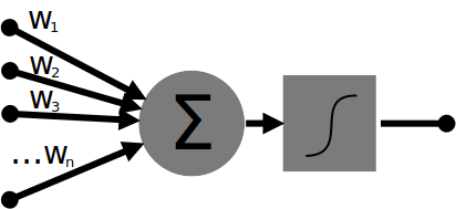
Each input value fed into a neuron is multiplied by specific weight value for that input source. The neuron then sums all of the multiplied input * weight values. This sum is then fed through an activating function (typically the Sigmoid Function) which determines the output value of the neuron, between 0 and 1 or -1 and 1. Neurons are arranged in a layered network, where the output from a given neuron is connected to one or more nodes in the next layer. This will be described in more detail with the first simple example. ANN are trained by feeding data through the network and observing the error, then adjusting the weights throughout the network based on the output error.

So why FANN? There’s certainly plenty of choices out there when it comes to creating ANNs. FANN is one of the most prevalent libraries for creating practical neural network applications. It is written in C but provides an easy-to-use C++ interface, among many others. Despite its reasonably friendly interface (the C++ interface could benefit from being more idiomatic), FANN can still be counted on to provide performance in both training and running modes. Mostly I’m using FANN because of its maturity and ubiquity, which usually results in better documentation (whether first or third party) and better long term support.

While using the latest stable version of FANN (2.2.0) for the first example in this post I ran into a bug in the C++ interface for the create_standard method of the neural_net object. This bug has persisted for about 6 years, and could have been around since the C++ interface was first introduced back in 2007. The last stable release (2.2.0) of FANN was in 2012, now over 4 years ago. There was a 5 year gap before that release too. The latest git snapshot seems to improve the ergonomics of the C++ interface a little, and includes unit tests. To install on a linux-based environment simply run the following commands (requires Git and CMake):

1
2
3
4

git clone git@github.com:libfann/fann.git
cd fann
mkdir build && cd build
cmake .. && make install

Another issue that might trip new FANN users up is includes and linking. FANN uses different includes to switch between different underlying neural network data types. Including fann.h or floatfann.h will cause FANN to use the float data type internally for network calculations, and should be linked with -lfann or -lfloatfann respectively. Likewise doublefann.h and -ldoublefann will cause FANN to use the double type internally. Finally, as a band-aid for environments that cannot use float, including fixedfann.h and linking with -lfixedfann will allow the excecution of neural networks using the int data type (this cannot be used for training). The header included will dictate the underlying type of fann_type. In order to use the C++ interface you must include one of the above C header files in addition to fann_cpp.h.

The most basic example for using a neural network is emulating basic boolean logic patterns. I’ll take the XOR example from FANN’s Getting Started guide and modify it slightly so that it uses FANN’s C++ interface instead of the C one. The XOR problem is an interesting one for neural networks because it is not linearly separable, and so cannot be solved with a single-layer perceptron.

The training code, train.cpp, which generates the neural network weights:

1
2
3
4
5
6
7
8
9
10
11
12
13
14
15
16
17
18
19
20
21
22
23
24
25
26

#include <array>
#include <fann.h>
#include <fann_cpp.h>
using uint = unsigned int;
int main() {
    // Neural Network parameters
    constexpr uint num_inputs = 2;
    constexpr uint num_outputs = 1;
    constexpr uint num_layers = 3;
    constexpr uint num_neurons_hidden = 3;
    constexpr float desired_error = 0.0001;
    constexpr uint max_epochs = 500000;
    constexpr uint epochs_between_reports = 1000;
    
    // Create the network
    const std::array<uint, 4> layers = {num_inputs, num_neurons_hidden, num_outputs};
    FANN::neural_net net(FANN::LAYER, num_layers, layers.data());
    net.set_activation_function_hidden(FANN::SIGMOID_STEPWISE);
    net.set_activation_function_output(FANN::SIGMOID_STEPWISE);
    
    net.train_on_file("xor.data", max_epochs, epochs_between_reports, desired_error);
    net.save("xor_float.net");
}

There aren’t too many changes from the original example here. I’ve defined an alias for unsigned int to save some typing, changed the const variables to constexpr, and moved the neuron counts for each layer into an array instead of passing them directly. One significant change I did make was to change the activation function from FANN::SIGMOID_SYMMETRIC to FANN::SIGMOID_STEPWISE. The symmetric function produces output between -1 and 1, while the other non-symmetric Sigmoids product an input between 0 and 1. The stepwise qualifier on the activation function I have used implies that it is an approximation of the Sigmoid function, so some accuracy is sacrificed for some gain in calculation speed. As we are dealing with discrete values at opposite ends of the scale, accuracy isn’t much of a concern. In reality for this example there is no difference between using either FANN::SIGMOID_SYMMETRIC or FANN::SIGMOID_STEPWISE, but there are applications where the activation function does affect the output. I encourage you to experiment with changing the activation function and observing the effect.

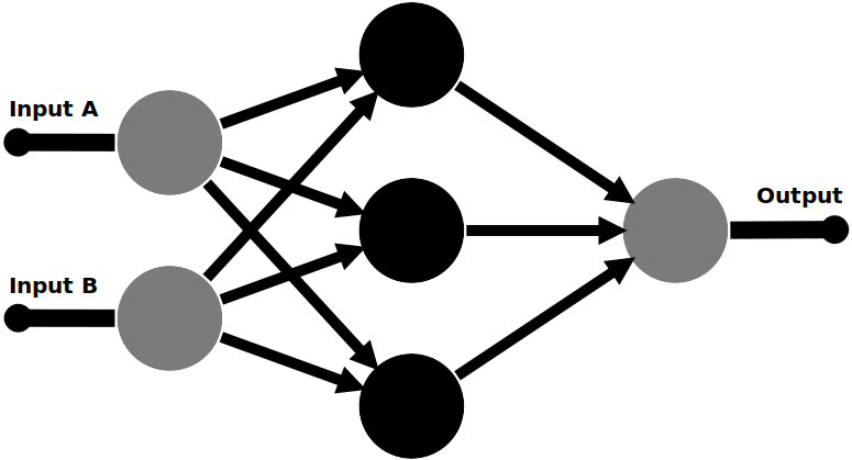
The network parameters in this training program describe a multi-layer ANN with an input layer, one hidden layer and an output layer. The input layer has two neurons, the hidden layer has three, and the output layer has one. The input and output layers obviously correspond to the desired number of inputs and outputs, but how is the number of hidden layer neurons or hidden layers calculated? Even with all of the research conducted on ANNs, this part is still largely driven by experimentation and experience. In general, most problems won’t require more than one hidden layer. The number of neurons has to be tweaked based on your problem; if you have too few you will probably see issues with poor fit or generalization, too many will mostly be a non-issue apart from driving up training and computation times.

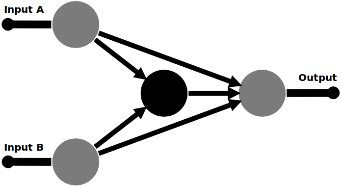
One optimization we can make to this network is to use the FANN::SHORTCUT network type instead of FANN::LAYER. In a standard multi-layer perceptron, all of the neurons in each layer are connected to all of the neurons in the next layer (see illustration above). With the SHORTCUT network type, each node in the network is connected to all nodes in all subsequent layers. In some cases (such as this one) shortcut connectivity can reduce the number of neurons required, because some layered neurons can be acting as pass-through neurons for subsequent layers. If we change the network type to FANN::SHORTCUT and reduce the number of hidden nodes to 1, the network topology becomes:

Fundamentally, this network produces exactly the same output as the layered network, but with fewer neurons.

The input data, xor.data:

1
2
3
4
5
6
7
8
9

4 2 1
0 0
0
0 1
1
1 0
1
1 1
0

Note the input data format. The first line gives the number of input/output line pairs in the file, the number of inputs to the network, and the number of outputs. Following that is the training test cases with alternating input and output lines. Values on each line are space-separated. I’ve changed the data from the original example to be based on logic levels of 0 and 1 instead of -1 and 1.

Finally, running the network with run.cpp:

1
2
3
4
5
6
7
8
9
10
11
12
13
14
15
16
17
18
19
20
21
22
23
24
25
26
27
28
29
30
31

#include <cstdlib>
#include <array>
#include <iostream>
#include <fann.h>
#include <fann_cpp.h>
int main(int argc, char const **argv) {
    // Parse command line input for values
    std::array<fann_type, 2> input{0.f, 1.f};
    if (argc > 2) {
        std::cout << "Got input parameters: ";
        for (int i = 1; i < 3; ++i) {
            input[i-1] = std::atof(argv[i]);
            std::cout << input[i-1] << " ";
        }
        std::cout << std::endl;
    } else {
        std::cout << "Using default input values: 0 1" << std::endl;
    }
    
    // Run the input against the neural network
    FANN::neural_net net("xor_float.net");
    
    fann_type* output = net.run(input.data());
    if (output != nullptr)
        std::cout << "output: " << *output << std::endl;
    else
        std::cout << "error, no output." << std::endl;
    return 0;
}

The first part of the main function is just parsing the command-line arguments for input values, so the network can be tested against multiple inputs without having to recompile the program. The second part of the program has been translated into more idiomatic C++ and updated to use the new and improved C++ API from the in-development FANN version (tentatively labeled 2.3.0). The neural network is loaded from the file produced by the training program, and executed against the input.

Note that in order to run this code you will need to download and install the latest development version of FANN from the project’s Github repository.

I created a simple script to compile the code, run the training, and test the network.

1
2
3
4
5
6
7

g++ -std=c++14 -Wall -Wextra -pedantic -lfann -o train train.cpp
g++ -std=c++14 -Wall -Wextra -pedantic -lfann -o run run.cpp
./train
./run 0 0
./run 1 1
./run 0 1
./run 1 0

Training Output:

1
2
3

Max epochs   500000. Desired error: 0.0001000000.
Epochs            1. Current error: 0.2512120306. Bit fail 4.
Epochs          168. Current error: 0.0000802190. Bit fail 0.

Running Output:

1
2
3
4
5
6
7
8

Got input parameters: 0 0 
output: 0.00792649
Got input parameters: 1 1 
output: 0.0101204
Got input parameters: 0 1 
output: 0.993475
Got input parameters: 1 0 
output: 0.990801

The outputs aren’t exactly 1 or 0, but that’s part of the nature of Artificial Neural Networks and the Sigmoid activation function. ANNs approximate the appropriate output response based on inputs and their training. If they are over-trained they will produce extremely accurate output values for data that they were trained against, but such over-fitted networks will be completely useless for generalizing in response to input data that the network was not trained against. Generalization is a key reason for using an ANN instead of a fixed function or heuristic algorithm, so over-fitting is something we want to avoid. This property of ANN output is also useful for obtaining a measure of confidence in results produced. In this case we can threshold the outputs of the neural network at 0.5 to obtain a discrete 0 or 1 logic level output. From the results we can see that the network does indeed mimic a logical XOR function.

How about another slightly more complex example? One of my favorite small data sets to play around with is the Iris data set from the UCI Machine learning repository. I modified the code I used for the XOR example above to increase the number of inputs, outputs and hidden neurons. The data set includes 4 inputs; sepal length, sepal width, petal length and petal width. The output is the class of the iris, which I have encoded as a 1.0 output on one of three outputs. The number of hidden neurons was increased through experimentation, 10 seemed like a reasonable start points.

The training code:

1
2
3
4
5
6
7
8
9
10
11
12
13
14
15
16
17
18
19
20
21
22
23
24
25
26

#include <array>
#include <fann.h>
#include <fann_cpp.h>
using uint = unsigned int;
int main() {
    // Neural Network parameters
    constexpr uint num_inputs = 4;
    constexpr uint num_outputs = 3;
    constexpr uint num_layers = 3;
    constexpr uint num_neurons_hidden = 10;
    constexpr float desired_error = 0.01;
    constexpr uint max_epochs = 500000;
    constexpr uint epochs_between_reports = 1000;
    
    // Create the network
    const std::array<uint, 4> layers = {num_inputs, num_neurons_hidden, num_outputs};
    FANN::neural_net net(FANN::LAYER, num_layers, layers.data());
    net.set_activation_function_hidden(FANN::SIGMOID);
    net.set_activation_function_output(FANN::SIGMOID);
    
    net.train_on_file("iris.data", max_epochs, epochs_between_reports, desired_error);
    net.save("iris_float.net");
}

The training data:

And to run the resulting network:

1
2
3
4
5
6
7
8
9
10
11
12
13
14
15
16
17
18
19
20
21
22
23
24
25
26
27
28
29
30
31
32
33
34
35
36
37
38
39
40
41
42
43
44
45
46
47
48
49
50
51
52
53
54
55
56
57
58
59
60
61
62
63
64
65
66

#include <cstdlib>
#include <array>
#include <vector>
#include <iostream>
#include <fstream>
#include <cstdint>
#include <iterator>
#include <algorithm>
#include <cassert>
#include <fann.h>
#include <fann_cpp.h>
int main() {
    // Load neural network from file created by train.cpp
    FANN::neural_net net("iris_float.net");
    
    // Load test values from file
    std::ifstream test_file("iris.data.test");
    uint32_t test_count = 0, input_count = 0, output_count = 0;
    test_file >> test_count >> input_count >> output_count;
    
    std::vector<std::array<float, 4>> input;
    input.resize(test_count);
    assert(input_count == 4);
    std::vector<std::array<float, 3>> expected_output;
    expected_output.resize(test_count);
    assert(output_count == 3);
    
    auto input_it = input.begin();
    auto expected_output_it = expected_output.begin();
    while (test_file.good() && input_it != input.end() && expected_output_it != expected_output.end()) {
        std::copy_n(std::istream_iterator<float>(test_file), input_count, input_it->begin());
        std::copy_n(std::istream_iterator<float>(test_file), output_count, expected_output_it->begin());
        ++input_it;
        ++expected_output_it;
    }
    
    // Run the input against the neural network
    uint32_t pass_count = 0, fail_count = 0;
    for (uint32_t i = 0; i < test_count; ++i) {
        fann_type* output = net.run(input[i].data());
        if (output != nullptr) {
            std::cout << "-- test " << i << " --" << std::endl;
            std::cout << "output:          " << output[0] << " " << output[1] << " " << output[2] << std::endl;
            std::cout << "expected output: " << expected_output[i][0] << " " << expected_output[i][1] << " " << expected_output[i][2] << std::endl;
            if (std::round(output[0]) == expected_output[i][0] &&
                std::round(output[1]) == expected_output[i][1] &&
                std::round(output[2]) == expected_output[i][2]) {
                ++pass_count;
            } else {
                ++fail_count;
            }
        } else {
            std::cout << "error, no output." << std::endl;
            ++fail_count;
        }
    }
    
    std::cout << "-----------------------------------------" << std::endl
        << "passed: " << pass_count << std::endl
        << "failed: " << fail_count << std::endl
        << "total:  " << pass_count + fail_count << std::endl
        << "-----------------------------------------" << std::endl;
    return 0;
}

The training output:

1
2
3

Max epochs   500000. Desired error: 0.0099999998.
Epochs            1. Current error: 0.2574429810. Bit fail 423.
Epochs          140. Current error: 0.0099833719. Bit fail 8.

In order to prove the generalization capacity of neural networks, I took 9 random input/output pairs from the training data set and put them into a second file iris.data.test (removing them from the iris.data training file). The program in run.cpp loads this data and runs the network against it. So bear in mind the results are against data that the network has never seen in training. The training data in iris.data.test follows the same format as the training files:

1
2
3
4
5
6
7
8
9
10
11
12
13
14
15
16
17
18
19

9 4 3
4.4 2.9 1.4 0.2
1 0 0
5.1 3.3 1.7 0.5
1 0 0
5.2 4.1 1.5 0.1
1 0 0
5.6 2.9 3.6 1.3
0 1 0
6.7 3.0 5.0 1.7
0 1 0
6.4 2.9 4.3 1.3
0 1 0
7.1 3.0 5.9 2.1
0 0 1
7.7 2.6 6.9 2.3
0 0 1
6.0 2.2 5.0 1.5
0 0 1

The output from running the network against the test data:

1
2
3
4
5
6
7
8
9
10
11
12
13
14
15
16
17
18
19
20
21
22
23
24
25
26
27
28
29
30
31
32

-- test 0 --
output:          1 0 0
expected output: 1 0 0
-- test 1 --
output:          1 5.43803e-08 7.23436e-34
expected output: 1 0 0
-- test 2 --
output:          1 0 0
expected output: 1 0 0
-- test 3 --
output:          4.68331e-10 0.999837 0.000162127
expected output: 0 1 0
-- test 4 --
output:          8.09432e-13 0.707596 0.32776
expected output: 0 1 0
-- test 5 --
output:          8.26562e-11 0.999368 0.000931072
expected output: 0 1 0
-- test 6 --
output:          1.56675e-14 0.00915556 0.990563
expected output: 0 0 1
-- test 7 --
output:          1.61667e-15 0.000615397 0.999422
expected output: 0 0 1
-- test 8 --
output:          1.40737e-13 0.186112 0.801713
expected output: 0 0 1
-----------------------------------------
passed: 9
failed: 0
total:  9
-----------------------------------------

In order to categorize the correctness of the output I rounded each output and compared it with the expected output for that input. Overall, the network correctly classified 9 of 9 random samples that it had never seen before. This is excellent generalization performance for a first attempt at such a problem, and with such a small training set. However, there is still room for improvement in the network; I did observe the ANN converging on a suboptimal solution a couple of times where it would only correctly classify about 30% of the input data and always produce 1.0 on the first output, no matter what the input. When I ran the best network against the training set, it would produce an misclassification rate of about 1-2% (2/141 was the lowest error rate I observed). This is a more realistic error rate than the 0% error rate of the small test data set.

Improving the convergence and error rates could be achieved by having more training data, adjusting the topography of the network (number of nodes/layers and connectivity), or changing the training parameters (such as reducing the learning rate). One facility offered by FANN which can make this process a little less experimental is cascade training which starts with a bare perceptron and gradually adds nodes to the network to improve its performance, potentially arriving at a more optimal solution.

With some experimentation I was able to remove 2 of the nodes from the network without visibly affecting its performance. Removing more nodes did increase the error slightly, and removing 5 nodes caused the network to sometimes fail completely to converge on a solution. I also experimented with reducing the desired error for training to 0.0001. This caused the network to become over-fitted: it would produce perfect results against the training data set (100% accuracy) but didn’t generalize as well for the data it hadn’t seen.

I found Artifical Neural Networks to be fairly easy to implement with FANN, and I have been very impressed by the performance obtained with minimal investment in network design. There are avenues to pursue in the future to further increase performance, but for most classification applications an error rate of 1-2% is very good.

This post is going to be a general background article on unique_ptr and how/why you should use it (if you are not already). In my current line of work I still deal with a large C++03 codebase, but with efforts ongoing to pull C++11 into the application I have spent a great deal of time thinking about how we can make the most out of C++11. One of the biggest wins is smart pointers and manual memory management, which are usable in C++03 with boost, but are so much more powerful in C++11 thanks to move semantics. I will focus on unique_ptr in this post as a start, but that doesn’t mean you shouldn’t also use the other smart pointer types included in C++11, shared_ptr and weak_ptr, when appropriate.

Anatomy Of A unique_ptr

The unique_ptr introduced with C++11 (based on boost::scoped_ptr) is conceptually very simple. It wraps a raw pointer to a heap-allocated object with RAII semantics, destroying the associated object with the unique_ptr (i.e. at the end of whatever scope it is declared in). Because object destruction is triggered by RAII, there is no runtime or memory overhead for unique_ptr compared to a raw pointer. There are 3 ways to bind an object instance to a unique_ptr:

• The constructor that takes a raw T*.

1

std::unique_ptr<MyClass> instance(new MyClass());

• With make_unique (the return value of which can be move-assigned).

1

auto instance = std::make_unique<MyClass>();

• By using the reset member function.

1
2

std::unique_ptr<MyClass> instance;
instance.reset(new MyClass());

There is only one way to destroy the object associated with the unique_ptr early, before the unique_ptr itself is destroyed.[1] Destroying the contained object early (before the unique_ptr itself is destroyed) can be triggered by calling the reset member function, which can also optionally take another raw pointer that the unique_ptr should subsequently take ownership of. However, before taking ownership of the new pointer it will always ensure the previous object is deleted first. If no new pointer is passed to reset, the unique_ptr will hold nullptr after the current object is deleted. The same logic applies to assignments; a unique_ptr can be move-assigned an object from another unique_ptr, or assigned nullptr. In both cases any object already held by the unique_ptr will be deleted before accepting the new value.

Using smart pointers is semantically the same as with raw pointers. The * and -> operators have both been overloaded to provide familiar mechanics for accessing the underlying object:

1
2
3

std::unique_ptr<MyClass> instance(new MyClass());
std::cout << instance->v << std::endl;
int y = (*instance).calculate();

In fact modern smart pointers in C++ go one further by defining an implicit bool conversion; so the == nullptr, == 0, == NULL, or whatever null-pointer constant your organization has chosen, can be excluded.

1
2
3
4

std::unique_ptr<MyClass> instance(new MyClass());
std::unique_ptr<MyClass> noinstance;
assert(instance); // `instance` is initialized and valid
assert(!noinstance); // `noinstance` is uninitialised and invalid

Block-Scoped Object Lifetimes

The time/space within the program between the creation and deletion of an object is the object’s lifetime: the part of the program for which the object is valid. With smart pointers, this is dictated by the owning smart pointer(s) controlling the object’s lifetime.

Consider the following C++03-ish example:

1
2
3
4
5

{
    MyClass* instance(new MyClass());
    // ... more code ...
    delete instance;
}

With C++11 and unique_ptr this becomes:

1
2
3
4

{
    std::unique_ptr<MyClass> instance(new MyClass());
    // ... more code ...
} // `instance` deallocated here automatically

Or better yet, using make_unique from C++14:

1
2
3
4

{
    auto instance = std::make_unique<MyClass>();
    // ... more code ...
} // `instance` deallocated here automatically

This concept can be extended with class scopes to yield a wider range of object lifetimes we can express using unique_ptr. For example, the traditional PIMPL pattern (simplified for this example):

1
2
3
4
5
6
7
8

class Outer {
public:
    Outer() : impl(new Inner()) {};
    ~Outer() { delete impl; }
    
private:
    Inner* impl;
}

With modern C++ this can be refactored to:

1
2
3
4
5
6
7

class Outer {
public:
    Outer() : impl(std::make_unique<Inner>()) {};
    
private:
    std::unique_ptr<Inner> impl;
}

Note we don’t even need to define a destructor anymore, because our impl object is automatically destroyed when the Outer object is destroyed.

Why Smart Pointers Instead Of Manual Memory Management?

I have had people ask this question when I have suggested using smart pointers instead of traditional manual memory management (using delete), because their existing code works perfectly fine and causes no leaks. The most obvious benefit of using smart pointers is avoiding memory leaks (shared_ptr reference cycles being an exception). But how does using smart pointers avoid leaks?

When manual memory management is done correctly it does indeed work, but it becomes more brittle over time as code is refactored and extended. As a simplified example, say we had some code like this hiding somewhere in our application:

1
2
3
4
5

{
    MyClass* instance = new MyClass();
    // ... more code ...
    delete instance;
}

Then, while adding a new feature, someone modifies the code so there are multiple places where a pointer is initialized with an instance of different types (using runtime polymorphism). In reality a mistake like this is much less obvious than in this example. This example intentionally shows very poor design to make the flaw more obvious.

1
2
3
4
5
6
7
8
9
10
11
12

{
    MyClass* instance = 0;
    if (someCondition) {
        instance = new SubclassA();
    }
    // ... more code ...
    if (someOtherCondition) {
        instance = new SubclassB();
    }
    // ... more code ...
    delete instance;
}

Whoops, we may have just caused a memory leak: if both conditions are true the first object assigned to instance is never deleted. We could fix this up by calling delete to dispose of the first object before we create the second if the instance pointer is not zero.

1
2
3
4
5
6
7
8
9
10
11
12
13

{
    MyClass* instance = 0;
    if (someCondition)
        instance = new SubclassA();
    // ... more code ...
    if (someOtherCondition) {
        if (instance != nullptr)
            delete instance;
        instance = new SubclassB();
    }
    // ... more code ...
    delete instance;
}

This sort of breakage can be very common when modifying code that uses traditional manual memory management techniques comprised of delete calls scattered throughout code. This error could have just as well been a double free due to over-application of delete. It could have also been a use after free error where the pointer is not reset to nullptr after deletion, and our program continues to use it unaware until suddenly Cthulhu starts wreaking havoc on our application. The more resilient modern technique to eliminate all of these simple errors is to apply smart pointers in these scenarios instead wherever possible. For example, if we rewrite the above original example using unique_ptr:

1
2
3
4

{
    auto instance = std::make_unique<MyClass>();
    // ... more code ...
} // `instance` automatically deleted here

With the same naive refactoring applied this would become:

1
2
3
4
5
6
7
8
9
10
11

{
    std::unique_ptr<MyClass> instance;
    if (someCondition) {
        instance.reset(new SubclassA()); // no delete here, `instance` starts out as `nullptr` automatically
    }
    // ... more code ...
    if (someOtherCondition) {
        instance.reset(new SubclassB()); // any previous object associated with `instance` delete here
    }
    // ... more code ...
} // `instance` automatically deleted here

And it Just Works™. No pitfalls to be seen here; the API of smart pointers does not allow an already held pointer to be overwritten without first triggering a release of the object associated with that pointer. It’s extremely difficult to screw up the usage of unique_ptr in these types of scenarios.

Raw Pointers/References And unique_ptr

So with the advent of smart pointers in modern C++ are we supposed to completely throw away raw pointers and references? Of course not!

Raw pointers and references still serve a purpose for referencing/accessing objects without affecting their lifetime. The usual rules apply: for raw pointers and references to be valid, the lifetime of the raw pointers/references must be a subset of the lifetime of the object being referred to. It is easier to align the lifetimes of both smart and raw pointers if RAII and scope are used to manage both.

Consider the following example:

1
2
3
4
5
6
7
8
9
10
11
12
13
14
15

{
    // Scope 1
    auto instance = std::make_unique<MyClass>();
    {
        // Scope 2
        MyClass* ptrA = instance.get();
        // ... some usage of ptrA ...
    }
    // ... more code ...
    {
        // Scope 3
        MyClass* ptrB = instance.get();
        /// ... some usage of ptrB
    }
}

The lifetimes in this example could be represented by the following Venn diagram:

Whereas if we got the lifetimes wrong and did something like this:

1
2
3
4
5
6
7
8
9
10
11
12
13
14
15
16

{
    // Scope 2
    MyClass* ptrA;
    {
        // Scope 1
        auto instance = std::make_unique<MyClass>();
        ptrA = instance.get();
        {
            // Scope 3
            MyClass* ptrB = instance.get();
            /// ... some usage of ptrB
        }
    }
    // ... some usage of ptrA ...
    // oops! ptrA is invalid because `instance` and the associated object no longer exist
}

The associated Venn diagram of the lifetimes would look more like this:

This would result in a use-after-free error when we try to access ptrA after the end of Scope 1, and possibly an application crash.

Smart Pointers For A Better Tomorrow

There are a multitude of safety and maintainability advantages when using smart pointers instead of traditional manual memory management with direct calls to delete. Using smart pointers won’t provide any immediate gratification over working delete code, but in the long term they make code much more resilient in the face of maintenance, refactoring and extension.

With the addition of shared_ptr, weak_ptr and move semantics from C++11 there should be few real scenarios which still require manual delete calls. Hopefully as C++ continues to develop and advance this will be ever more true. delete is still useful to have in your C++ development toolbox, but it should be a tool of last resort.

Stay tuned for a follow-up post on shared_ptr and weak_ptr.

Update:
[1] Thanks to /u/immutablestate on reddit for pointing out that assignment operations can also trigger an early release of an object held by a unique_ptr.

Thanks to /u/corysama and /u/malaprop0s for other corrections.

Recently I’ve been working on a little side project in the form of a C++ k-means clustering library. Development recently reached a point where the project was functionally complete, so I began to look for other areas to improve. One such improvement was adding Continuous Integration (CI) via Travis CI.

Travis CI is the de-facto standard for CI-as-a-service for Github projects. It automatically detects when new code is pushed to a Github repository (including on branches) and will execute whatever jobs are set up for that repository (builds, testing, static analysis, etc.). According to stats available publicly uptake of CI-as-a-service is relatively low for C++. This could be due to C++ projects not having CI, or it might just be that C++ projects (like Firefox and Dolphin) have their own infrastructure and so don’t need or want to rely on a third party service.

At this point I’m assuming you’re already sold on the idea of CI, because another entire blog post could be devoted to explaining why you should use CI and what you should do with it. This post focuses on the technical how question: specifically, with regards to building modern C++ code on Travis.

Basic Configuration

Travis is very easy to get set started with. Add a configuration file (.travis.yml) to the repository with some information about the type of build(s) to run, and enable Travis CI on Github: under Integrations globally, and under Webhooks and services in the settings for each repository.

The basic .travis.yml for a C++ project looks something like this:

1
2
3
4
5
6
7
8
9
10
11

# Enable C++ support
language: cpp
# Compiler selection
compiler:
  - clang
  - gcc
# Build steps
script:
  - mkdir build
  - cd build
  - cmake .. && make

This is a good start. It gets us builds against GCC 4.6.3 and Clang 3.4 on Ubuntu 12.04 Precise. Travis uses these parameters to construct a “Build Matrix”. The build matrix is effectively a table of all of the possible combinations of build options specified in the configuration. In a simple configuration like this it consists only of different compilers and operating systems. We have specified one operating system and two compilers, so we get 1 * 2 = 2 different builds. In a more complex configuration we can specify different environments, build procedures and other variations to ramp up the number of configurations tested in each job. The Build Matrix in Travis CI is very powerful and flexible.

Travis CI Environment Limitations

Hold on, did I say GCC 4.6? Clang 3.4?

This won’t do. This won’t do at all.

GCC declared itself feature complete at 4.8.1 according to the C++11 feature matrix, but <regex> was missing until GCC 4.9. So for modern C++ I would expect to be using GCC 4.9 at minimum. We get lucky with Clang; 3.4 has full C++11 support, and even feature-complete C++14 support. Great, so I can at least get a build going using Clang.

cmake .. && make
CMake Error at CMakeLists.txt:1 (cmake_minimum_required):
  CMake 3.0 or higher is required.  You are running version 2.8.7

CMake 2.8? I chose 3.0 for my project as a compromise between being on the bleeding edge and having to support an ancient toolset. The version offered by Travis’ build slaves is over 4 years old.

For other languages that Travis is popular with (e.g. Javascript, Ruby, Python) Travis (the company) backports the latest runtimes, and provides a range of the latest versions for user to choose from. For example, for Python they provide 2.6, 2.7, 3.2, 3.3, 3.4, 3.5 and a nightly python build. Even Rust projects get to build against its stable, beta and nightly channels with the latest compiler or range of specific versions. No such support is provided for building C and C++ code on Travis: all we get by default is the compilers shipped with the platform.

This project has only a single code dependency on OpenCV 2.x, which is thankfully available in the apt repositories for Ubuntu 12.04. Other projects may not be so fortunate with the libraries and kernels available on such a mature version of Ubuntu.

Building Modern C++ on Travis (C++11/C++14)

So is this the end of the road for building modern C++ projects on Travis? Fortunately it is not. Other people have already run into all of these same problems and provided solutions or hints which we can use to set up a working C++11/14 build.

One way of getting a more up-to-date toolchain is to opt into the “beta” Ubuntu 14.04 Trusty build environment. To use the Trusty build environment add the following to your .travis.yml:

1
2
3

# Ubuntu 14.04 Trusty support
sudo: required
dist: trusty

Unfortunately this is not as advantageous as it first appears. It gets us GCC 4.8.4 and Clang 3.5.0 and CMake 2.8.12. Again, the version of Clang available is sufficient for building modern C++ code, but the GCC and CMake versions are still a bit further behind than we would like. At this point I conceded the CMake version, since my CMakeLists files worked with CMake 2.8.

So how can we get even more up to date dependencies over what the platform offers? As the Travis build environment is Ubuntu based, is it possible to add specific external PPAs for up-to-date dependencies. In this case we need to add two PPAs for our compilers, one for LLVM and one for GCC. Unfortunately there is currently an open issue for adding the Trusty LLVM ppa to Travis’ whitelist (at the time of writing), so in order to use an up-to-date LLVM compiler I had to also revert to the Ubuntu 12.04 build environment.

1
2
3
4
5
6
7
8
9
10
11

addons:
  apt:
    sources:
    # add PPAs with more up-to-date toolchains
    - ubuntu-toolchain-r-test
    - llvm-toolchain-precise-3.6
    packages:
    # install toolchains
    - gcc-5
    - g++-5
    - clang-3.6

Now, if this is added to the .travis.yml and a build is kicked off Travis will still use the old compiler, because it is simply setting the compiler environment variables to g++ or clang++ respectively, which doesn’t pick up the newly install non-default versions. At first I toyed with reconfiguring the default with Ubuntu’s update-alternatives tool, but there were a few problems around using this for the clang build. Instead I settled on an environment variable juggling technique suggested on StackOverflow.

I mentioned earlier that the build matrix can be used to generate a suite of different builds that are all triggered in the same job. Adding specific configurations can be done via the matrix.include property in .travis.yml. Each item in the sequence (denoted by -) details a different build configuration. This configuration could specify a compiler/runtime, environment variables, build steps ppa sources, packages, etc. I configured the build matrix to be made up of 4 builds total, GCC 4.9 and 5.x (currently 5.2 from the ubuntu-toolchain-r-test ppa) and Clang 3.6 and 3.7.

1
2
3
4
5
6
7
8
9
10
11
12
13
14
15
16
17
18
19
20
21
22
23
24
25
26
27
28
29
30
31
32
33
34
35
36

matrix:
  include:
    - compiler: gcc
      addons:
        apt:
          sources:
            - ubuntu-toolchain-r-test
          packages:
            - g++-4.9
      env: COMPILER=g++-4.9
    - compiler: gcc
      addons:
        apt:
          sources:
            - ubuntu-toolchain-r-test
          packages:
            - g++-5
      env: COMPILER=g++-5
    - compiler: clang
      addons:
        apt:
          sources:
            - ubuntu-toolchain-r-test
            - llvm-toolchain-precise-3.6
          packages:
            - clang-3.6
      env: COMPILER=clang++-3.6
    - compiler: clang
      addons:
        apt:
          sources:
            - ubuntu-toolchain-r-test
            - llvm-toolchain-precise-3.7
          packages:
            - clang-3.7
      env: COMPILER=clang++-3.7

Conclusion

Building modern C++ projects on Travis is entirely possible, if a little tricky to set up. With the apt addon for Travis and a custom build matrix we can target multiple compilers for every build. Github integration means automatic builds on every branch and pull request. And best of all, it’s free for open source projects. If you have an open source project C++ project on Github I would suggest there is no reason not to make use of Travis.

The final configuration I ended up with for my project is available on github, and you can see the associated build on Travis.